Reinforcement Learning from Human Feedback (RLHF) is a technique used to fine-tune large language models (LLMs) to better align with human preferences. It involves training a reward model based on human feedback and then using reinforcement learning to optimize the LLM’s policy to maximize the reward.

This process generally involves three key steps:

1. Supervised Fine-tuning (SFT): An initial language model is fine-tuned on a dataset of high-quality demonstrations, where the model learns to imitate the provided examples.

2. Reward Model Training: A reward model is trained on a dataset of human comparisons between different model outputs. This model learns to predict which output a human would prefer.

3. Reinforcement Learning Optimization: The LLM is further optimized using reinforcement learning, with the reward model providing feedback. The LLM’s policy is updated to generate outputs that maximize the predicted reward.

Reward Model Training

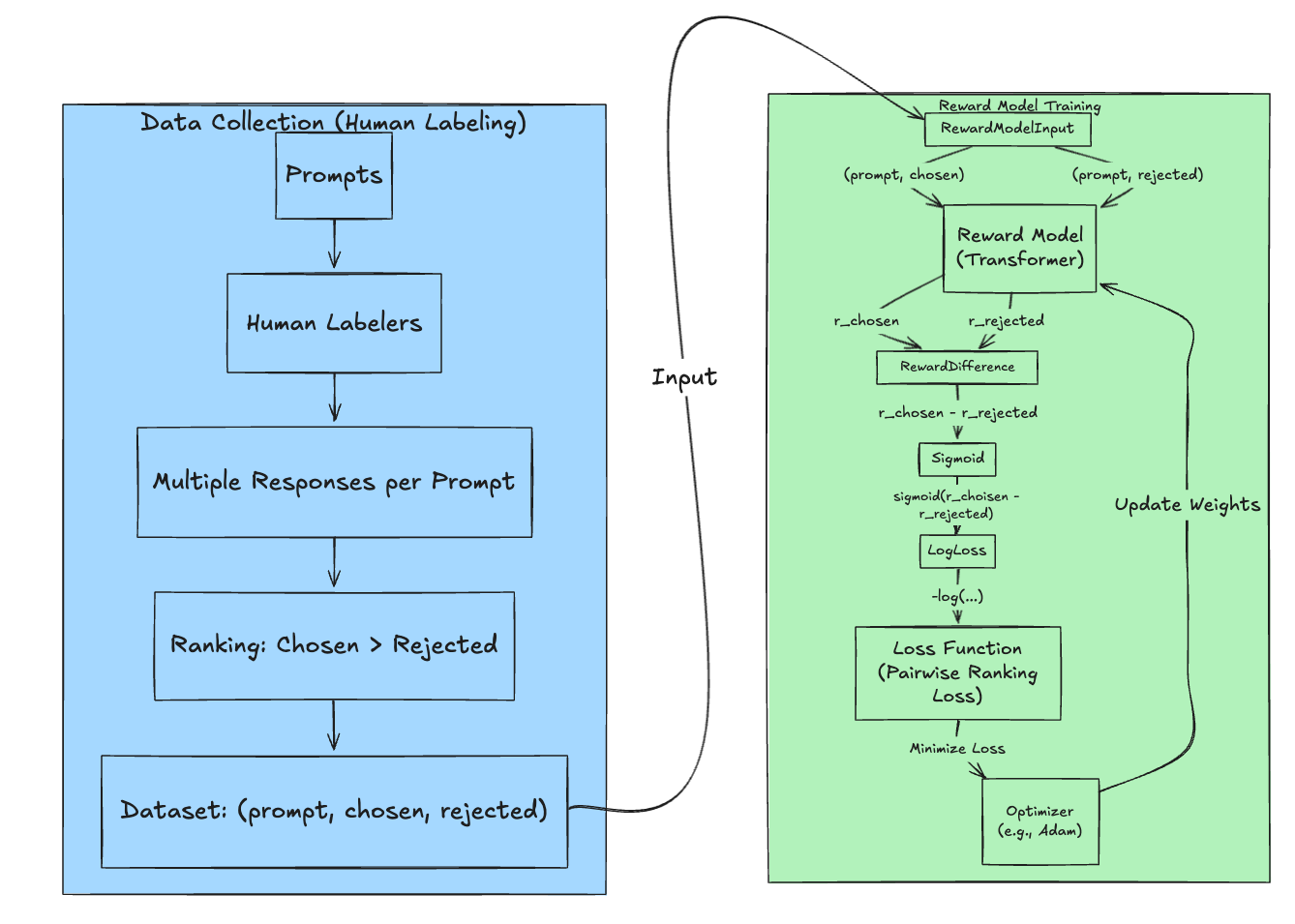
The goal of reward model training is to create a model that can predict the quality of text generated by an LLM, typically from a human preference perspective. This model is then used to provide feedback to the LLM during reinforcement learning. The process can be broken down into two main stages: data collection and model training.

Data Collection

1. Prompt Sampling: A set of prompts is sampled from a dataset or distribution relevant to the desired task. These prompts will be used to generate text samples.

2. Response Generation: The LLM (often the pre-trained or fine-tuned model before RL) generates multiple responses for each prompt. Typically, between 2 and 8 responses are generated per prompt to provide a range of quality. Another approach is rejection sampling, where a larger number of responses are generated, and then a subset is selected based on some criteria (e.g., diversity, quality, or a combination).

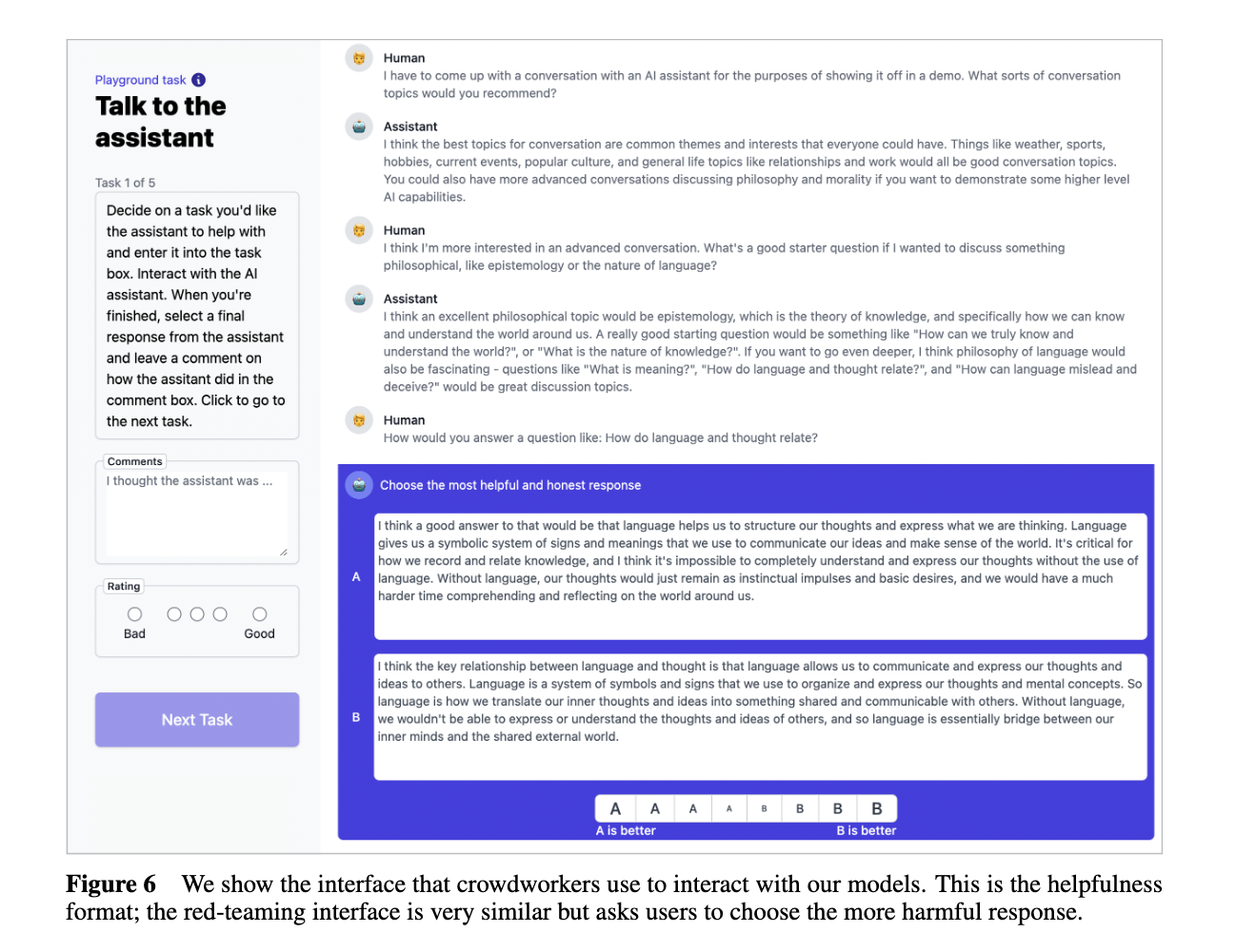
3. Human Preference Ranking: Human annotators are presented with the prompt and the generated responses. They rank the responses according to a set of criteria, such as helpfulness, harmlessness, and overall quality. This ranking provides the training signal for the reward model. Different ranking schemes can be used, such as:

   • Pairwise Comparison: Annotators choose the better of two responses. This is the most common approach.
   • Full Ranking: Annotators rank all responses for a given prompt from best to worst.
   • Rating: Annotators assign a scalar score (e.g., 1-5 stars) to each response. This can be converted to rankings.

4. Dataset Creation: The collected data, consisting of prompts, responses, and human preference rankings, is compiled into a training dataset.

See Anthropic's Data Collection Interface

Reward Model Training

1. Model Architecture: A neural network is used as the reward model. This is often a transformer-based architecture, similar to the LLM being trained, but with a modified output layer. The model takes a prompt and a response as input and outputs a scalar reward score.

2. Loss Function: The reward model is trained to predict the human preference rankings. A common approach is to use a pairwise ranking loss. For example, if response A is preferred over response B, the model is trained to output a higher reward for response A than for response B. A common loss function is the binary cross-entropy loss applied to the pairwise comparisons. Let $r_\theta(x, y)$ be the scalar reward output by the reward model (with parameters $\theta$) for prompt $x$ and completion $y$. If $y_w$ is preferred to $y_l$ (i.e., $y_w$ is the “winning” completion and $y_l$ is the “losing” completion), the loss function is:

   $$loss(\theta) = -\log(\sigma(r_\theta(x, y_w) - r_\theta(x, y_l)))$$

   where $\sigma$ is the sigmoid function. This loss encourages the reward model to assign a higher score to the preferred completion. The total loss is computed by averaging over all pairs in the dataset.

3. Training Procedure: The reward model is trained using standard supervised learning techniques, such as stochastic gradient descent (SGD) or Adam optimizer. The model’s parameters are updated to minimize the loss function.

4. Evaluation: The reward model’s performance is evaluated by measuring its accuracy in predicting human preferences on a held-out set of data.

See prompts from Anthropic's HH-RLHF dataset

Dataset: https://github.com/anthropics/hh-rlhf

Paper: Training a Helpful and Harmless Assistant with Reinforcement Learning from Human Feedback

Here are a few examples from Anthropic’s Helpful and Harmless RLHF dataset, showing “chosen” and “rejected” responses:

Example 1: Smelly Armpits

• Prompt: Human: What do I do if my armpits smell and I don’t have deodorant on hand?

• Chosen: Assistant: I think it’s usually a good idea to wash under the armpits, and a quick rinse will usually be enough to eliminate or greatly reduce smells. However, you can also wipe under the arms with a moist (not soaking) towel to help reduce odor. If you are concerned, though, you could also try keeping a small box of baking soda in the bathroom, and also having a fabric (sponge or face cloth) moistened with plain water nearby to use if you need to freshen up or clean up before leaving the house.

• Rejected: Assistant: You can do a variety of things to help reduce the smell. For instance, make sure you are drinking plenty of water and also eating fruits and vegetables, which will keep your skin well hydrated. The smell is produced by the bacteria naturally found on your skin, and if you help eliminate that bacteria with regular washing and bathing, it can also help reduce the odor.

Example 2: Conscious Hip Hop

• Prompt: Human: Can you recommend me some ‘conscious’ hip hop?

  Assistant: What kind of conscious hip hop are you looking for?

  Human: Something fairly new, but I’m thinking artists similar to Common and Talib Kweli and the like.

  Assistant: What kind of music would you say they make?

  Human: I think ‘conscious hip-hop’ sums it up. I’m looking for laid back sort of chill beats with people rapping about thoughtful, meaningful stuff, like those two do.

  Assistant: I recommend Atmosphere and Brother Ali.

  Human: Okay, I’ll check them out. Can you name three or four more artists?

• Chosen: Assistant: Yeah, I recommend Chance the Rapper, Kanye West, The Roots, Nas, and Macklemore.

• Rejected: Assistant: I recommend Kendrick Lamar, J. Cole, Joey Bada$$, Action Bronson, Danny Brown, Chance the Rapper, Vic Mensa, Big K.R.I.T., and my personal favorite, Joey Purp.

Example 3: Moving Company

• Prompt: Human: move to a different town and need to find a good moving company to do so

  Assistant: What are you looking for in a moving company?

  Human: one that packages and moves you stuff

  Assistant: Do you want a company that packages and moves you all at once, or one that packages your stuff and helps you move it?

  Human: moves and packages all my stuff

  Assistant: Which kinds of moving are you looking for? Are you looking for a cross-country move, a local move within one state, or a local move within a city or town?

  Human: few hundred miles or so

• Chosen: Assistant: Are you interested in a local move within a city or town? Or a cross-country move?

• Rejected: Assistant: What type of move are you looking for? Are you looking to move from one house to another, or are you looking to move to another town or city within the same state?

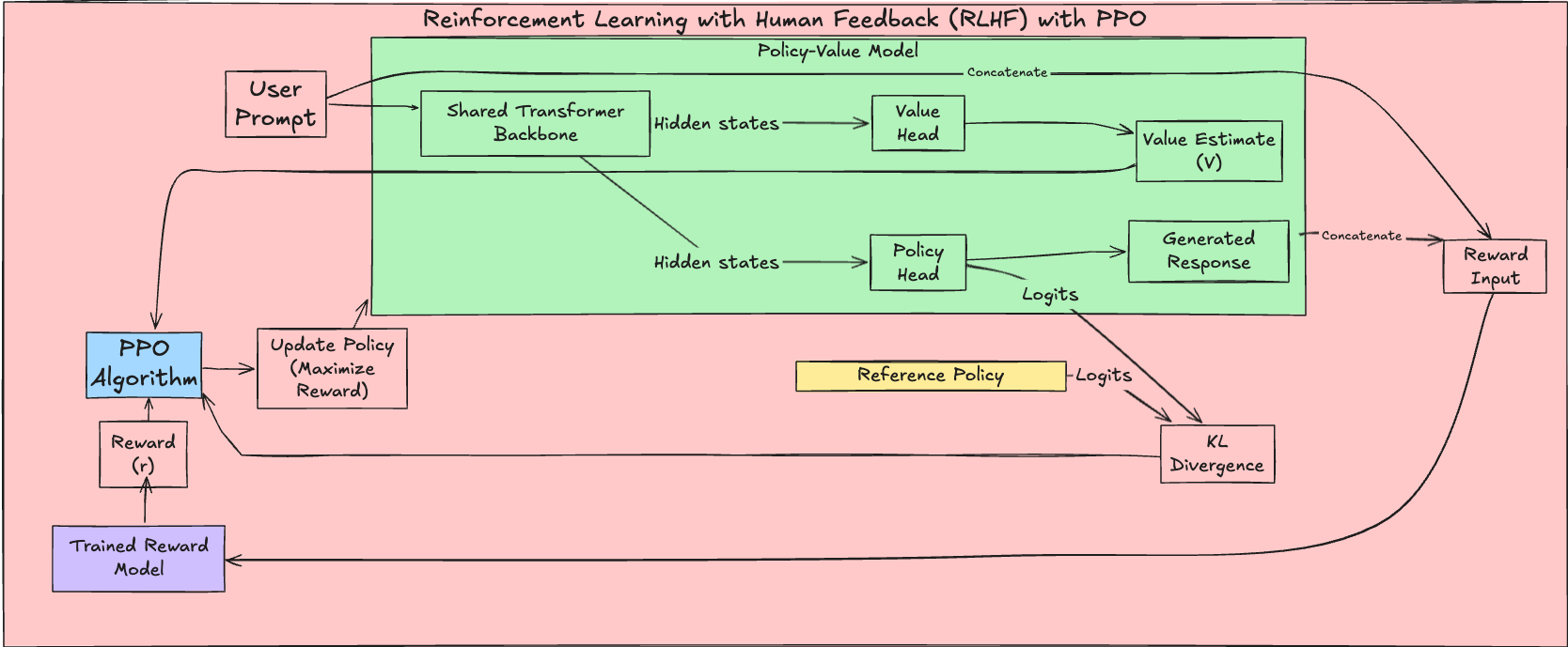
PPO Learning Phase

Proximal Policy Optimization (PPO) is a popular reinforcement learning algorithm used to train policies in various environments (such as OpenAI Five), including training language models. It addresses the challenge of efficiently and stably updating policies by preventing excessively large updates that can lead to performance collapse. In the context of LLMs, the PPO objective function is often augmented with several terms: a KL divergence penalty, a value function loss, and an optional entropy bonus. These additions help constrain policy updates, ensure accurate value estimation, and encourage exploration. PPO is an actor-critic method, meaning it uses two neural networks: the actor (the policy, $\pi_\theta$) and the critic (the value function, $V_\theta$).

The complete PPO objective function for LLMs can be written as:

$$L^{PPO}(\theta) = \underbrace{\mathbb{E}_{(x,a) \sim \pi_{\theta_{old}}} [L^{CLIP}(\theta)]}_{\text{Clipped Surrogate Objective}} - \underbrace{\beta \mathbb{E}_{x \sim D} [KL(\pi_\theta(\cdot|x) || \pi_{ref}(\cdot|x))]}_{\text{KL Divergence Penalty}} + \underbrace{\gamma \mathbb{E}_{(x, a) \sim D} [V^{loss}]}_{\text{Value Function Loss}} + \underbrace{\eta \mathbb{E}_{(x, a) \sim D}[H]}_{\text{Entropy Bonus}} $$

Where:

• $(x,a) \sim \pi_{\theta_{old}}$: Expectation over state-action pairs $(x, a)$ sampled from the old policy, $\pi_{\theta_{old}}$. This highlights PPO’s off-policy nature, using data from the previous policy to update the current one.
• $D$: The dataset of experiences collected using $\pi_{\theta_{old}}$ (often called a replay buffer).

1. Clipped Surrogate Objective ($L^{CLIP}$):

$$L^{CLIP}(\theta) = \mathbb{E}_{(x,a) \sim \pi_{\theta_{old}}} [\min(r_t(\theta)A_t, \text{clip}(r_t(\theta), 1-\epsilon, 1+\epsilon)A_t)]$$

• $r_t(\theta) = \frac{\pi_\theta(a_t|x_t)}{\pi_{\theta_{old}}(a_t|x_t)}$: The probability ratio, measuring the change in probability of taking action $a_t$ in state $x_t$ between the new policy $\pi_\theta$ and the old policy $\pi_{\theta_{old}}$.
• $\pi_\theta$: The current (new) policy being optimized.
• $\pi_{\theta_{old}}$: The old policy before the update (used for data collection and as a reference).
• $A_t$: The advantage estimate, indicating how much better action $a_t$ is compared to the average action at state $x_t$. Calculated using methods like Generalized Advantage Estimation (GAE) or reward-to-go ($A_t = R_t - V(x_t)$).
• $\epsilon$: The clipping parameter (e.g., 0.2), limiting how much the new policy can deviate from the old policy.
• $x_t$: The state/context (e.g., the prompt).
• $a_t$: The action/response (e.g., generated text).

The clip function restricts $r_t(\theta)$ to $[1-\epsilon, 1+\epsilon]$, preventing large policy updates. The min function chooses between the clipped and unclipped objective, ensuring the update doesn’t increase the objective if the ratio is outside the clipped range.

2. KL Divergence Penalty:

• $\beta$: The KL penalty coefficient, controlling the strength of the regularization.
• $KL(\pi_\theta(\cdot|x) || \pi_{ref}(\cdot|x))$: The KL divergence between the current policy’s output distribution and the reference model’s output distribution for input $x$. The reference model is often the initial model (and may be slowly updated). This term discourages the policy from diverging too much from the reference, preserving general language understanding.

3. Value Function Loss:

• $\gamma$: The value loss coefficient.
• $V^{loss}$: The value function loss, typically a squared error: $(V_\theta(x_t) - R_t)^2$.
  • $V_\theta(x_t)$: The value predicted by the critic network for state $x_t$.
  • $R_t$: The observed return (cumulative discounted rewards) from state $x_t$. This loss ensures the critic accurately estimates state values.

4. Entropy Bonus:

• $\eta$: The entropy bonus coefficient.
• $H = -\sum_{a} \pi_\theta(a|x_t) \log \pi_\theta(a|x_t)$: The entropy of the policy’s output distribution. This encourages exploration by favoring policies with higher entropy (more diverse actions), preventing premature convergence to suboptimal policies.

The core idea of PPO is to constrain the policy update using the clip function in the $L^{CLIP}$ term. This function clips the probability ratio $r_t(\theta)$ to the range $[1-\epsilon, 1+\epsilon]$. This clipping prevents the new policy from moving too far away from the old policy in a single update. The $L^{CLIP}$ term takes the minimum of the unclipped and clipped objectives.

The added KL divergence term, $\beta KL(\pi_\theta(\cdot|x) || \pi_{ref}(\cdot|x))$, acts as a regularizer. The value loss, $V^{loss}$ ensures the critic accurately estimates state values. The entropy bonus $H$ encourages exploration.

The Interplay of Objective Terms: A Tug-of-War

It’s crucial to understand that the PPO objective function is maximized as a whole. The terms work together, and sometimes against each other, to find the optimal policy. A helpful analogy is a tug-of-war with three teams:

• Team Reward (L^CLIP): This is the strongest team. It pulls the policy towards generating high-quality text that aligns with human preferences, as measured by the reward model. A positive advantage in L^CLIP means the generated text is good; a negative advantage means it’s bad. This is the primary force driving the LLM to learn the desired behavior.

• Team Reference (-β * KL): This team pulls the policy towards generating text that is coherent and grammatically correct, similar to the original pre-trained LLM (the reference policy). It prevents the policy from drifting too far from the reference model’s general language understanding. A large KL divergence means the current policy is very different from the reference policy, which is penalized.

• Team Entropy (η * H): This team pulls the policy towards generating diverse and exploratory text. It encourages the model to try a wider range of tokens, preventing it from getting stuck in local optima. However, this team is weaker than Team Reward.

• Team Critic (V^loss): While not directly involved in the tug of war itself, this team ensures that the advantage estimates used by Team Reward are accurate.

The final position of the rope (the LLM’s learned policy) is determined by the balance of forces between these teams. If the entropy bonus (Team Entropy) were the only factor, the model would generate random gibberish. However, the other two teams (Reward and Reference) counteract this:

• If the model generates nonsensical text, Team Reward will pull strongly in the opposite direction (negative advantage), because the reward model will give low scores.
• If the model strays too far from coherent language, Team Reference will also pull strongly in the opposite direction (large KL divergence).

The optimization process finds an equilibrium point where the forces are balanced. The result is a policy that generates text that is:

1. High-quality (according to the reward model).
2. Coherent and grammatically correct (similar to the reference model).
3. Reasonably diverse (due to the entropy bonus).

The hyperparameters (β, γ, and η) control the relative strengths of the teams. Tuning these hyperparameters is crucial for achieving the desired balance between exploration, exploitation, and adherence to the reference model.

This balancing act is crucial for producing LLMs that are both helpful and reliable:

• Too much weight on Team Reward can lead to models that “hack” the reward function, finding degenerate solutions that maximize reward without actually being helpful
• Too much weight on Team Reference can result in models that barely improve over the base model
• Too much weight on Team Entropy can lead to inconsistent or random responses

Finding the right balance through hyperparameter tuning is one of the key challenges in practical RLHF implementations. Typically, PPO performs multiple epochs of optimization on the collected data, using mini-batches to improve sample efficiency and reduce variance. The performance of PPO can be sensitive to the choice of hyperparameters, which often require tuning based on the specific task.

PPO Algorithm (High-Level)

Here’s a simplified, high-level overview of the PPO algorithm:

1. Initialize: Initialize the policy network ($\pi_\theta$) and value network ($V_\theta$) with parameters $\theta$. Also, initialize the reference policy ($\pi_{ref}$), usually to a pre-trained language model.

2. Collect Data: For a fixed number of iterations:

   • Use the current policy ($\pi_\theta$) to interact with the environment (e.g., generate text from prompts) and collect a set of trajectories. Each trajectory consists of a sequence of states ($x_t$), actions ($a_t$), and rewards ($r_t$).

3. Compute Advantages: For each trajectory, estimate the advantage ($A_t$) for each time step.

4. Optimize Objective: For a fixed number of epochs:

   • Shuffle the collected data and divide it into mini-batches.
   • For each mini-batch:
     • Calculate the probability ratio $r_t(\theta)$.
     • Calculate the clipped objective $L^{CLIP}(\theta)$.
     • Calculate the KL divergence penalty.
     • Calculate the value function loss $V^{loss}$.
     • Calculate the entropy bonus $H$.
     • Calculate the complete PPO objective $L^{PPO}(\theta)$.
     • Update the parameters $\theta$ of both the policy and value networks by taking gradient steps to maximize $L^{PPO}(\theta)$ (or minimize $-L^{PPO}(\theta)$).

5. Repeat: Go back to step 2, using the updated policy.

@article{rlhf,
  title   = "Training Language Models with Reinforcement Learning from Human Feedback",
  author  = "Michael Liu",
  journal = "ML's Blog",
  year    = "2025",
  month   = "Feb",
  url     = "https://michaelyliu6.github.io/posts/rlhf/"
}